Validation Case: Open Water Test – Potsdam Propeller

The aim of this validation is to compare the simulation results performed in SimScale using the proprietary solver, Multi-purpose, with the experimental data published by SVA Potsdam under the study Potsdam Propeller Test Case (PPTC)\(^1\).

The objective is to test the Multi-purpose solver’s ability to compute the thrust, torque, and propeller efficiency under open water test conditions.

Geometry

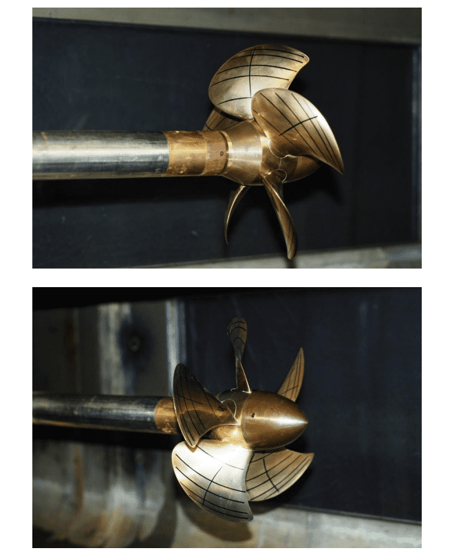
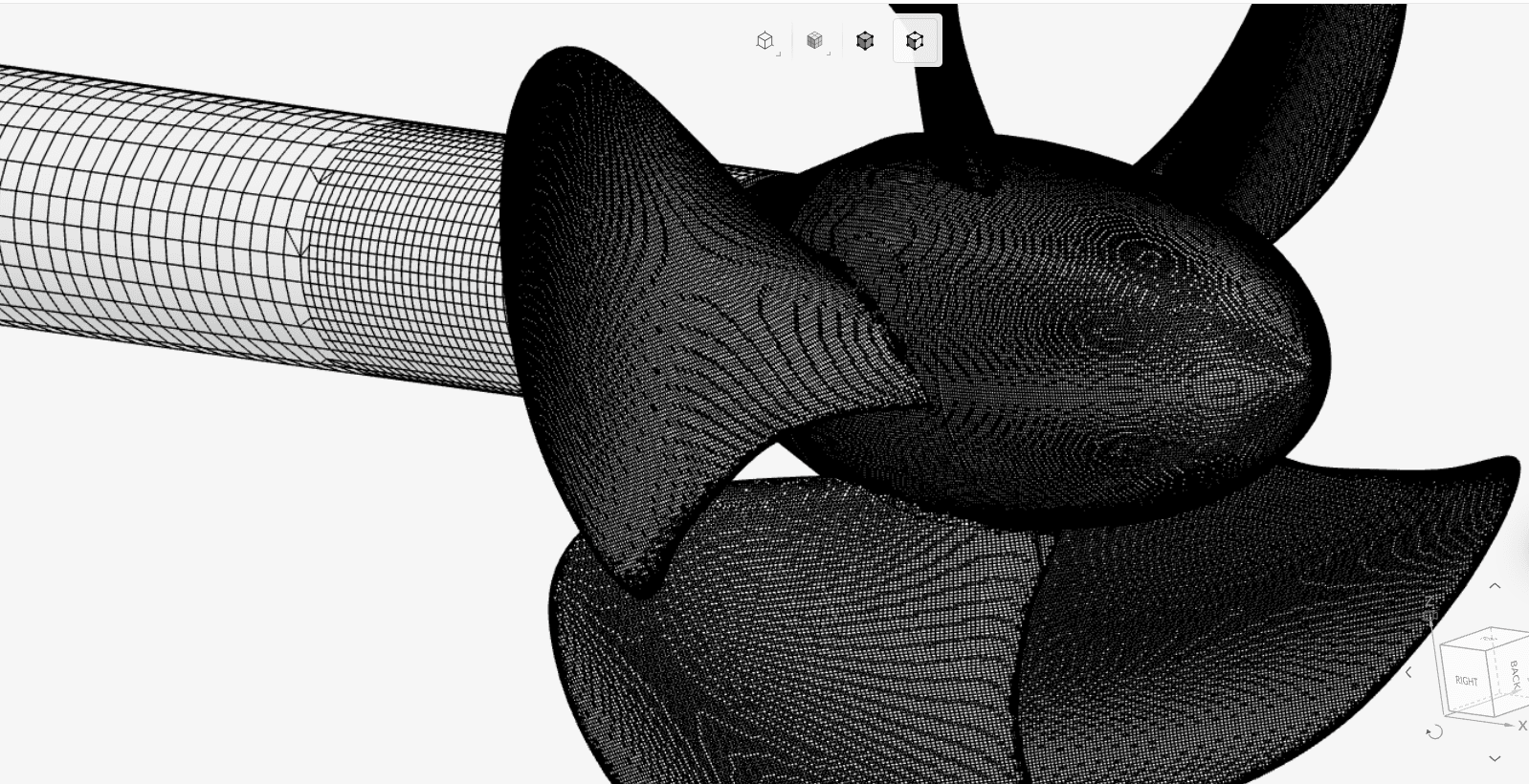
The Propeller model VP1304 can be downloaded from the SVA PPTC smp’11 Workshop. For simulation purposes in SimScale, an external flow volume is created around the propeller to replicate a propeller immersed under water. The original Propeller VP1304 as mentioned in the SVA report\(^1\) is as shown in Figure 1:

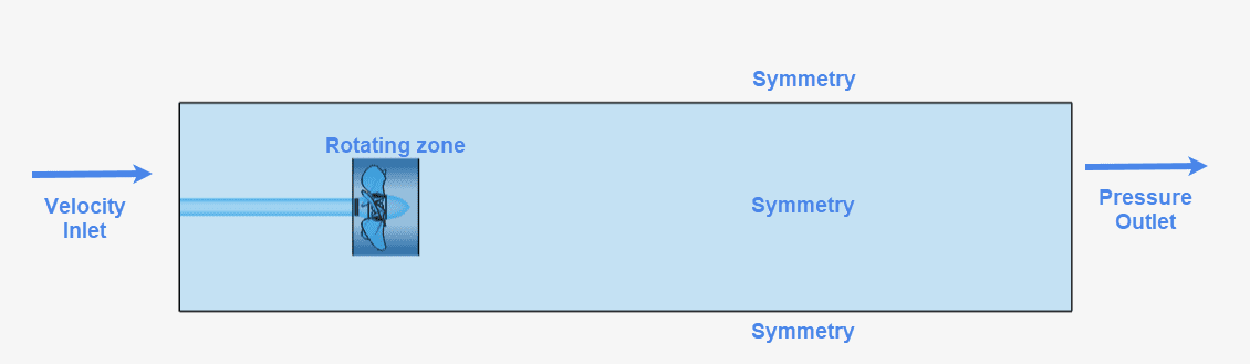
And the schematic is as follows:

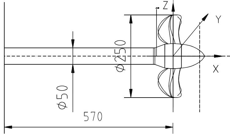
The propeller diameter is 0.25 \(m\), shaft diameter is 0.05 \(m\). The propeller blades are placed 0.57 \(m\) from the inlet.

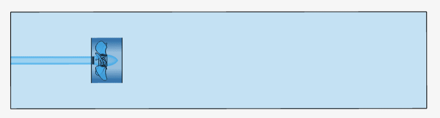
The CAD model used for validation purposes in SimScale is as follows:

Analysis Type and Mesh

Analysis Type: Steady-state, Multi-purpose with k-epsilon turbulence model.

Mesh and Element Types:

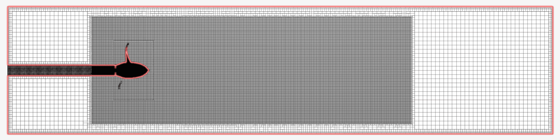
The mesh was created with SimScale’s Multi-purpose mesh type, which is a body-fitted structured mesh. An automatic sizing definition was defined with two additional region refinements for the wake region and around the rotating region, as well as one surface refinement to capture the blade profiles accurately.

Mesh Type	Fineness	Target Cell Size (surface refinement for rotor) \([m]\)	Target Cell Size (region refinement for wake) \([m]\)	Target Cell Size (region refinement for rotating zone) \([m]\)	Number of cells	Element Type
Automatic with region refinements	7	1e-3	5e-3	4e-3	22210996	3D Hexahedral

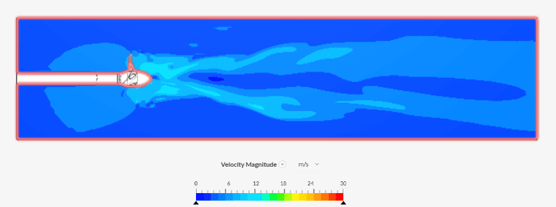
The resulting mesh is captured in Figures 4 and 5. Figure 4 shows cell distribution on a mid-plane while Figure 5 shows a closeup view of the surface refinements applied on the rotor.

Simulation Setup

Material

Fluid:

• Water
  • Kinematic viscosity \((\mu)\): 9.58e-7 \(m^2/s\)
  • Density \((\rho)\): 997.71 \(kg/m^3\)

Boundary Conditions

Figure 4 shows the schematic of the boundary conditions applied:

A total of 11 inlet velocities were tested for the same angular velocity.

Boundary Condition	Value
Velocity inlet \([m/s]\)	1.762 2.17 2.594 2.995 3.418 3.89 4.359 4.725 5.207 5.603 5.903
Pressure outlet \([Pa]\)	0 (Guage static pressure)
Symmetry	–
Rotating zone (MRF)	94.25 \(rad/s\) angular velocity (15 revolutions per second) in the negative x-axis

Result Comparison

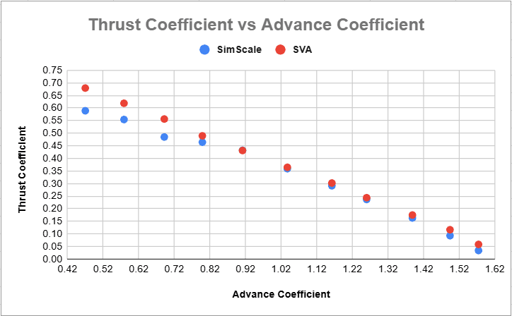
The result output for thrust and torque exerted by the propeller and the propeller efficiency obtained from the SimScale simulation are compared with the experimental measurements reported in the SVA study\(^1\).

Thrust

Thrust values exerted by the propeller VP1304 for the 11 input velocities were obtained by adding the pressure and viscous forces acting on the rotor (hub + blades) in the x direction.

For thrust \((T)\), the thrust coefficient is calculated as:

$$K_T = \frac{T}{\rho \times n^2 \times D^4} \tag{1}$$

A quantity called Advance coefficient is used for comparison, which is given by

$$J = \frac{v}{n \times D}$$

Where

• \(v\) is the inlet velocity \([m/s]\),
• \(n\) is the number of revolutions per second,
• \(D\) is the propeller diameter \([m]\).

Velocity \([m/s]\)	Advance Coefficient	Thrust, Simscale \([N]\)	Thrust Coefficient, SimScale	Thrust Coefficient, SVA	Error %
1.762	0.469867	516.5	0.5890	0.6791	-13.274
2.17	0.578666	486	0.5542	0.6187	-10.427
2.594	0.691733	425	0.4846	0.5562	-12.869
2.995	0.798666	407.07	0.4642	0.4895	-5.1809
3.418	0.911466	378.845	0.4320	0.4312	0.18104
3.89	1.03733	314.75	0.3589	0.3645	-1.5485
4.359	1.1624	255.21	0.2910	0.3020	-3.6561
4.725	1.26	207.52	0.2366	0.2437	-2.9113
5.207	1.38853	143.3	0.1634	0.175	-6.6184
5.603	1.49413	81.43	0.0928	0.1166	-20.404
5.903	1.57413	29.78	0.0339	0.0583	-41.781

Torque

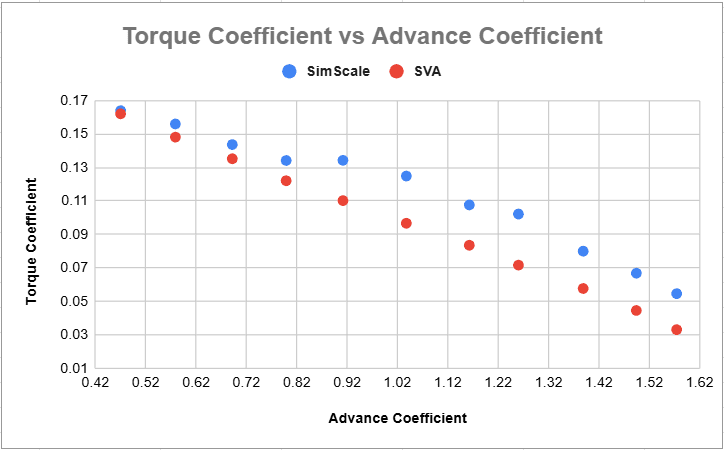
Torque values exerted by the propeller VP1304 for the 11 input velocities were obtained by calculating total moments (sum of pressure and viscous moments) acting on the rotor (hub + blades) in the x-direction.

For torque \((Q)\), the thrust coefficient is calculated as:

$$K_Q = \frac{Q}{\rho \times n^2 \times D^5} \tag{2}$$

Velocity \([m/s]\)	Advance Coefficient	Torque, Simscale \([Nm]\)	Torque Coefficient, SimScale	Torque Coefficient, SVA	Error %
1.762	0.469867	35.94	0.1639	0.1620	1.1469
2.17	0.578666	34.2	0.1560	0.1481	5.3200
2.594	0.691733	31.5	0.1436	0.1352	6.2723
2.995	0.798666	29.415	0.1341	0.1220	9.9070
3.418	0.911466	29.44	0.1342	0.1102	21.853
3.89	1.03733	27.375	0.1248	0.0966	29.178
4.359	1.1624	23.6	0.1076	0.0835	28.861
4.725	1.26	22.4	0.1021	0.0716	42.575
5.207	1.38853	17.535	0.0799	0.0577	38.605
5.603	1.49413	14.65	0.0668	0.0445	49.891
5.903	1.57413	11.975	0.0546	0.0331	64.904

Propeller Efficiency

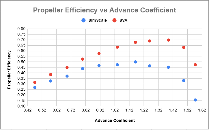
Propeller efficiency\((\eta)\) for the 11 input velocities was obtained using equation 3:

$$ \eta = \frac{K_T}{K_Q} \times \frac{J}{2 \pi} \tag{3}$$

Velocity \([m/s]\)	Advance Coefficient	Efficiency, SimScale	Efficiency, SVA	Error %
1.762	0.469867	0.2686	0.3145	-14.593
2.17	0.578666	0.3271	0.3854	-15.107
2.594	0.691733	0.3713	0.45	-17.478
2.995	0.798666	0.4397	0.525	-16.234
3.418	0.911466	0.4666	0.575	-18.837
3.89	1.03733	0.4745	0.6333	-25.069
4.359	1.1624	0.5001	0.6770	-26.131
4.725	1.26	0.4644	0.6895	-32.647
5.207	1.38853	0.4514	0.6979	-35.307
5.603	1.49413	0.3304	0.6312	-47.652
5.903	1.57413	0.1557	0.475	-67.208

Last updated: December 4th, 2025