Documentation
The aim of this validation is to compare the simulation results performed in SimScale using the compressible flow feature in its proprietary solver, Multi-purpose, with the simulation results in the study done by NASA titled, “Mach 2.0 Flow Over a 15 Degree Wedge\(^1\)” as well as the analytical results \(^2\).
The objective is to test the Multi-purpose solver’s ability to compute supersonic inviscid flows and in particular to capture oblique shock waves.
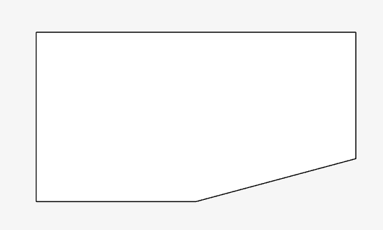
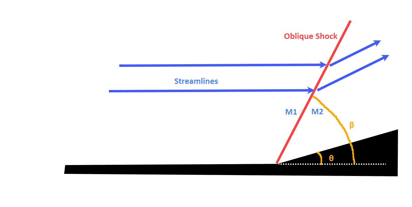
The geometry replicates a flow domain with an inviscid wedge. It has a tiny thickness to represent a two-dimensional flow. The geometry is inspired from the schematic\(^1\) as shown in Figure1:
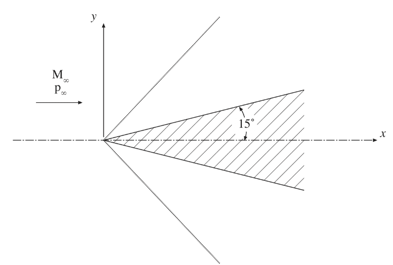
For simulation purposes, since the wedge is symmetric about the x-axis only, one-half of the wedge is considered in the CAD geometry.
Analysis Type: Steady-state, Multi-purpose with k-epsilon and Compressible model
Mesh and Element Types:
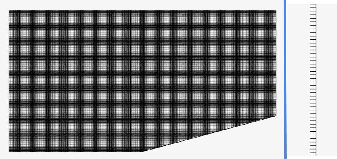
The mesh was created with SimScale’s Multi-purpose mesh type, which is a body-fitted structured mesh. A manual sizing definition relative to the CAD was used.
| Mesh Type | Minimum Cell Size | Maximum Cell Size | Cell Size on Surfaces | Number of cells | Element Type |
| Manual | 1e-5 (relative to CAD) | 0.004 (relative to CAD) | 0.0025 (relative to CAD) | 61868 | 3D Hexahedral |
Fluid:
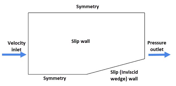
Figure 4 shows the schematic of boundary conditions applied
| Boundary Condition | Value |
| Velocity inlet \([m/s]\) | 686 (Fixed value with 527.4 \(K\) total temperature) |
| Pressure outlet \([Pa]\) | 101325 (Fixed absolute static pressure) |
| Slip wall | 1. Wedge to represent the inviscid boundary 2. Front and back faces to replicate a 2D flow |
| Symmetry | 1. Upstream portion at the bottom 2. Top face |
The symmetry boundary condition is used to simulate only one-half of the wedge (see Figure 1).
The total temperature at the inlet was calculated using the isentropic total temperature equation:
$$ T_t = T \left(1+ \frac{\gamma\ – 1}{2} M^2 \right) \tag{1}$$
All the variable definitions can be found in Table 3.
The ratios for the Mach number, temperature, pressure, and density after and before the shock are given by the equations using wave theory.
$$ \frac{P_2}{P_1} = 1+ \frac{2\gamma}{\gamma+1}(M_1^2sin^2 \beta\ – 1) \tag{2}$$
$$ \frac{\rho_2}{\rho_1} = \frac{(\gamma+1)M_1^2sin^2 \beta}{(\gamma-1)M_1^2sin^2 \beta\ + 2} \tag{3}$$
$$ \frac{T_2}{T_1} =\frac{P_2}{P_1}\frac{\rho_1}{\rho_2} \tag {4}$$
$$ M_2 = \frac{1}{sin(\beta-\theta)} \sqrt{\frac{1+\frac{\gamma\ – 1}{2}M_1^2sin^2 \beta}{\gamma M_1^2sin^2 \beta\ – \frac{\gamma\ – 1}{2}}} \tag{5}$$
The shock angle \(\beta\) is calculated using the equation
$$ \tan \theta = 2 \cot \beta \frac{M_1^2sin^2 \beta\ – 1 }{M_1^2(\gamma\ + \cos 2 \beta) + 2} \tag{6}$$
Where,
| Variable | Definition |
| \(M\) | Mach number |
| \(T\) | Temperature |
| \(P\) | Pressure |
| \(\rho\) | Air density |
| \(\gamma\) | Specific heat ratio |
| Subscripts 1, 2 | 1= before shock, 2 = after shock |
| \(\beta\) | Oblique shock angle |
| \(\theta\) | Wedge angle |
The result output from SimScale simulation is compared with the analytical results \(^2\) as well as the Mach number contours obtained from the NASA study \(^1\).
To compute and compare the before and after shock quantities, probe points were added as shown in Figure 6 before the simulation run.
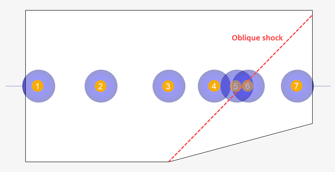
Using equations 2, 3, 4, and 5 the ratios of pressure, density, temperature, and Mach number are respectively compared against those obtained using probe points 5 and 6. These are given below:
| Quantity | Analytical | SimScale | Error [%] |
| Static pressure ratio | 2.1947 | 2.185 | -0.44 |
| Density ratio | 1.7289 | 1.7239 | -0.289 |
| Temperature ratio | 1.2694 | 1.267 | -0.189 |
| Mach number ratio | 0.72285 | 0.7239 | 0.1457 |
| Oblique shock angle | 45.34° | ~45° | ~0 |
As it can be derived the Multi-purpose solver was able to accurately match the nature of the oblique shock as the ratios of the involved quantities before and after the shock compare well.
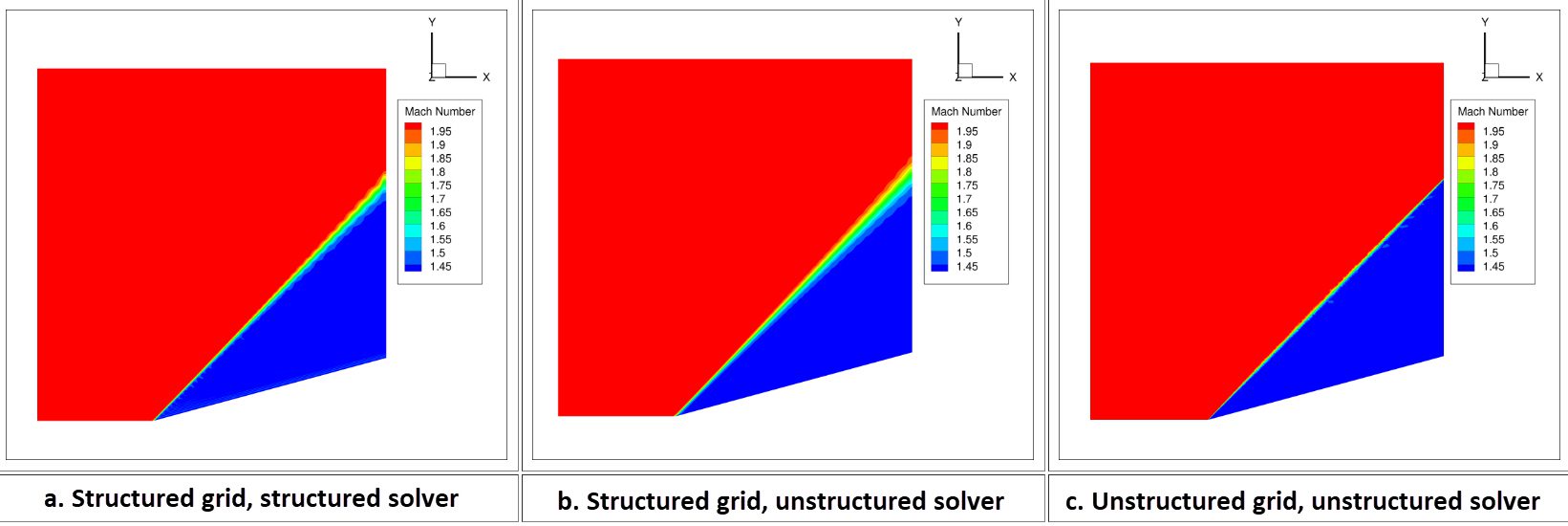
The NASA study\(^1\) compared eight separate cases using a combination of structured/unstructured grids with structured/unstructured solvers.
Depending on how the grid is clustered the shock wave is thin near the tip of the wedge and smears as it moves away from the wedge. This shock smearing is caused by the increase in the grid cell sizes away from the wedge surface. The solution obtained by the unstructured solver on the unstructured grid shows a very thin shock wave over the entire domain (Figure 7.c.). This is because the unstructured grid is clustered near the shock line throughout the domain.
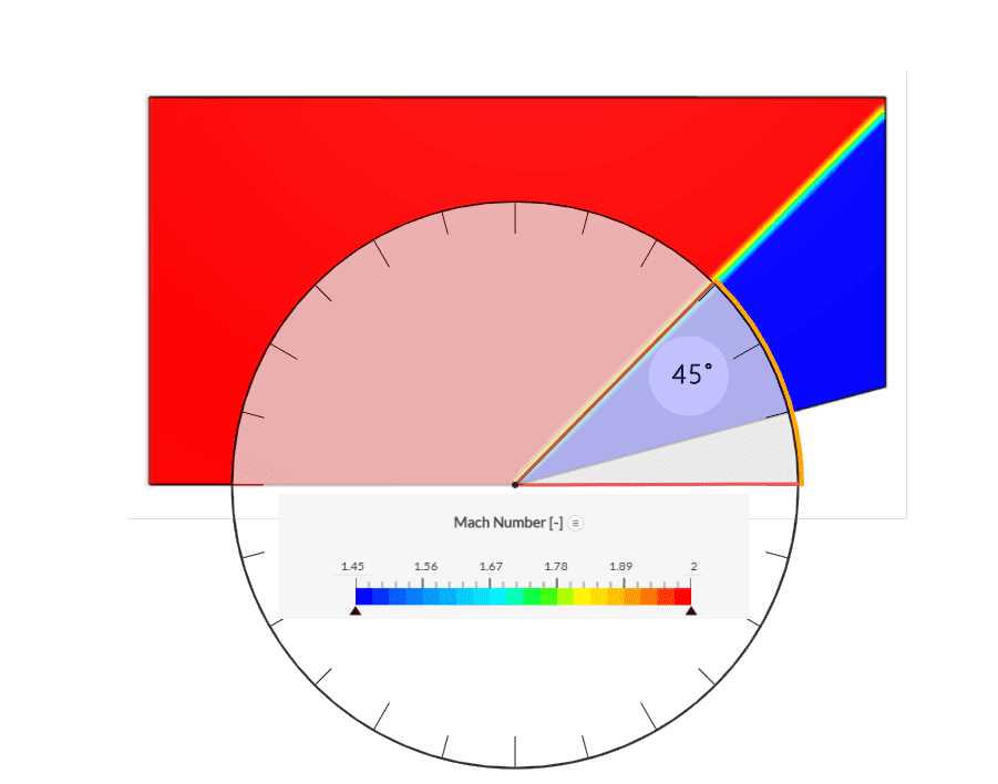
The Mach number contours obtained using SimScale’s Multipurpose solver show a similar trend as observed in Figure 8. The shock is thin at the tip and shows slight smearing as we move away. Further studies performed with finer mesh showed a decreasing diffusion trend and thinner shock.
The oblique shock is captured at an angle of ~45°. The legend was adjusted to match with those from the NASA study for ideal comparison.
Note
If you still encounter problems validating your simulation, then please post the issue on our forum or contact us.
Last updated: March 14th, 2025
We appreciate and value your feedback.
Sign up for SimScale
and start simulating now